spaudiopy.plot

Plotting helpers.

import numpy as np
import matplotlib.pyplot as plt
plt.rcParams['axes.grid'] = True

import spaudiopy as spa

Functions

`compare_ambi`(Ambi_A, Ambi_B)	Compare A and B format signals.
`decoder_performance`(hull, renderer_type[, ...])	Shows amplitude, energy, spread and angular error measures on grid.
`doa`(azi, zen[, p, size, c, alpha, fs, ...])	Direction of Arrival, with optional p(t) scaling the size.
`freq_resp`(freq, amp[, TODB, smoothing_n, ...])	Plot magnitude of frequency response over time frequency f.
`hrirs_ild_itd`(hrirs[, plevels, pclims, ...])	Plot ILDs and ITDs of HRIRs.
`hull`(hull[, simplices, mark_invalid, title, ...])	Plot loudspeaker setup and valid simplices from its hull object.
`hull_normals`(hull[, plot_face_normals, ...])	Plot loudspeaker setup with vertex and face normals.
`polar`(theta, r[, TODB, rlim, title, ax])	Polar plot (in dB) that allows negative values for r.
`set_aspect_equal3d`([ax, XYZlim])	Set 3D axis to equal aspect.
`sh_bar`(x_nm[, TODB, centered, num_groups, ...])	Barplot over SH channels.
`sh_coeffs`(F_nm[, sh_type, azi_steps, ...])	Plot spherical harmonics coefficients as function on the sphere.
`sh_coeffs_overlay`(F_nm_list[, sh_type, ...])	Overlay spherical harmonics coefficients plot.
`sh_coeffs_subplot`(F_nm_list[, titles, fig])	Plot spherical harmonics coefficients list as function on the sphere.
`sh_rms_map`(F_nm[, TODB, w_n, sh_type, ...])	Plot spherical harmonic signal RMS as function on the sphere.
`spectrum`(x, fs[, ylim, scale_mag])	Positive (single sided) amplitude spectrum of time signal x.
`spherical_function`(f, azi, zen[, title, ax])	Plot function 1D vector f over azi and zen.
`spherical_function_map`(f, azi, zen[, TODB, ...])	Plot function 1D vector f over azi and zen, can also convert to dB.
`transfer_function`(freq, H[, title, xlim])	Plot transfer function H (magnitude and phase) over time frequency f.
`zeropole`(b, a[, zPlane, title])	Plot Zero Pole diagram from a and b coefficients.

spaudiopy.plot.spectrum(x, fs, ylim=None, scale_mag=False, **kwargs)[source]

Positive (single sided) amplitude spectrum of time signal x. kwargs are forwarded to plot.freq_resp().

Parameters:

x (np.array, list of np.array) – Time domain signal.
fs (int) – Sampling frequency.

spaudiopy.plot.freq_resp(freq, amp, TODB=True, smoothing_n=None, xlim=(20, 24000), ylim=(-30, None), title=None, labels=None, ax=None)[source]

Plot magnitude of frequency response over time frequency f.

Parameters:

f (frequency array)
amp (array_like, list of array_like)
TODB (bool) – Plot in dB.
smoothing_n (int) – Forwarded to process.frac_octave_smoothing()

Examples

See spaudiopy.sph.binaural_coloration_compensation()

spaudiopy.plot.transfer_function(freq, H, title=None, xlim=(10, 25000))[source]: Plot transfer function H (magnitude and phase) over time frequency f.

spaudiopy.plot.zeropole(b, a, zPlane=False, title=None)[source]: Plot Zero Pole diagram from a and b coefficients.

spaudiopy.plot.compare_ambi(Ambi_A, Ambi_B)[source]: Compare A and B format signals.

spaudiopy.plot.spherical_function(f, azi, zen, title=None, ax=None)[source]: Plot function 1D vector f over azi and zen.

spaudiopy.plot.sh_coeffs(F_nm, sh_type=None, azi_steps=5, el_steps=3, title=None, ax=None, cbar=True)[source]

Plot spherical harmonics coefficients as function on the sphere. Evaluates the inverse SHT.

Examples

See spaudiopy.sph

spaudiopy.plot.sh_coeffs_subplot(F_nm_list, titles=None, fig=None, **kwargs)[source]

Plot spherical harmonics coefficients list as function on the sphere. kwargs are forwarded to spaudiopy.plt.sh_coeffs.

Examples

See spaudiopy.sph

spaudiopy.plot.sh_coeffs_overlay(F_nm_list, sh_type=None, azi_steps=5, el_steps=3, title=None, ax=None)[source]

Overlay spherical harmonics coefficients plot.

Examples

See spaudiopy.plot.sh_coeffs

spaudiopy.plot.sh_rms_map(F_nm, TODB=False, w_n=None, sh_type=None, n_plot=50, title=None, clim=[0, None], ax=None)[source]

Plot spherical harmonic signal RMS as function on the sphere. Evaluates the maxDI beamformer, if w_n is None.

Parameters:

F_nm (((N+1)**2, S) numpy.ndarray) – Matrix of spherical harmonics coefficients, Ambisonic signal.
TODB (bool) – Plot in dB.
w_n (array_like) – Modal weighting of beamformers that are evaluated on the grid.
sh_type (‘complex’ or ‘real’ spherical harmonics.)
n_plot (int) – Plotting precision (grid degree).

Examples

See spaudiopy.sph.src_to_sh

spaudiopy.plot.spherical_function_map(f, azi, zen, TODB=False, title=None, clim=(None, None), ax=None)[source]

Plot function 1D vector f over azi and zen, can also convert to dB.

Examples

See spaudiopy.parsa.sh_beamform

spaudiopy.plot.sh_bar(x_nm, TODB=True, centered=False, num_groups=1, s=250, vf=4, clim=None, xticklabels=None, title=None, ax=None)[source]

Barplot over SH channels.

Parameters:

x_nm (array_like) – C x L.
TODB (TYPE, optional) – DESCRIPTION. The default is True.
centered (TYPE, optional) – DESCRIPTION. The default is False.
num_groups (TYPE, optional) – Plot gourps. The default is 1.
s (TYPE, optional) – Scatter plot size. The default is 250.
vf (TYPE, optional) – Vertical ratio. The default is 4.
clim (TYPE, optional) – DESCRIPTION. The default is None.
xticklabels (TYPE, optional) – DESCRIPTION. The default is None.
title (TYPE, optional) – DESCRIPTION. The default is None.
fig (TYPE, optional) – DESCRIPTION. The default is None.

Returns:

None.

spaudiopy.plot.hull(hull, simplices=None, mark_invalid=True, title=None, draw_ls=True, ax_lim=None, color=None, clim=None, ax=None)[source]

Plot loudspeaker setup and valid simplices from its hull object.

Parameters:

hull (decoder.LoudspeakerSetup)
simplices (optional)
mark_invalid (bool, optional) – mark invalid simplices from hull object.
title (string, optional)
draw_ls (bool, optional)
ax_lim (float, optional) – Axis limits in m.
color (array_like, optional) – Custom colors for simplices.
clim ((2,), optional) – vmin and vmax for colors.

Examples

See spaudiopy.decoder

spaudiopy.plot.hull_normals(hull, plot_face_normals=True, plot_vertex_normals=True)[source]: Plot loudspeaker setup with vertex and face normals.

spaudiopy.plot.polar(theta, r, TODB=True, rlim=None, title=None, ax=None)[source]

Polar plot (in dB) that allows negative values for r.

Examples

See spaudiopy.sph.bandlimited_dirac()

spaudiopy.plot.decoder_performance(hull, renderer_type, azi_steps=5, ele_steps=3, show_ls=True, title=None, **kwargs)[source]

Shows amplitude, energy, spread and angular error measures on grid. For renderer_type={‘VBAP’, ‘VBIP’, ‘ALLRAP’, ‘NLS’}, as well as {‘ALLRAD’, ‘ALLRAD2’, ‘EPAD’, ‘MAD’, ‘SAD’}. All kwargs are forwarded to the decoder function.

References

Zotter, F., & Frank, M. (2019). Ambisonics. Springer Topics in Signal Processing.

Examples

See spaudiopy.decoder

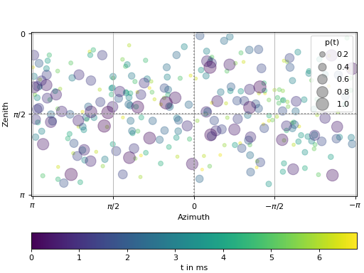
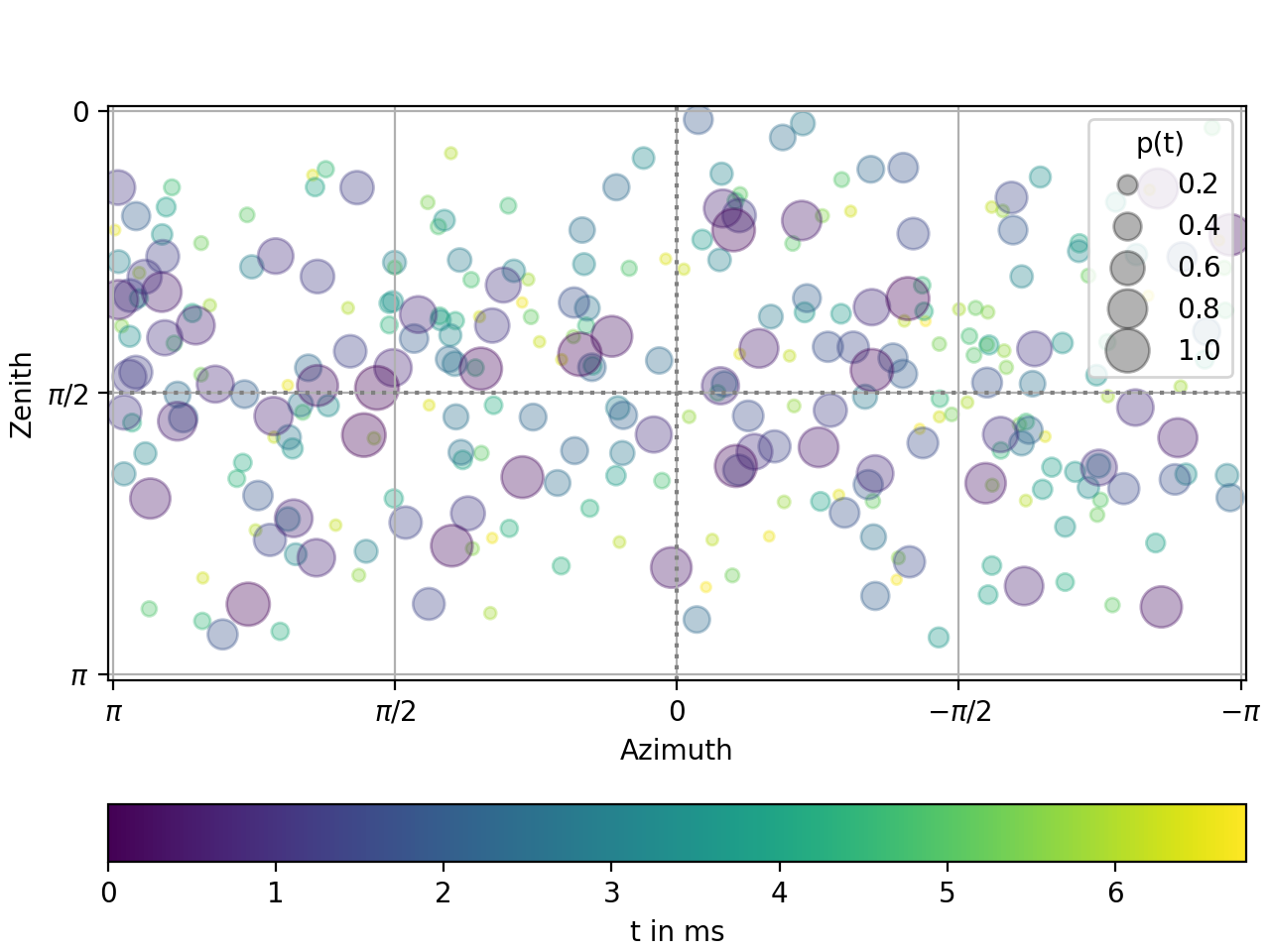
spaudiopy.plot.doa(azi, zen, p=None, size=250, c=None, alpha=None, fs=None, title=None, ltitle=None, ax=None)[source]

Direction of Arrival, with optional p(t) scaling the size.

Examples

n = 300
fs = 44100
t_ms = np.linspace(0, n/fs, n, endpoint=False) * 1000  # t in ms

x = np.random.randn(n)
y = np.random.randn(n)
z = np.random.randn(n)
azi, zen, r = spa.utils.cart2sph(x, y, z)

ps = 1 / np.exp(np.linspace(0, 3, n))
spa.plot.doa(azi, zen, ps, fs=fs, ltitle="p(t)")

(png, hires.png, pdf)

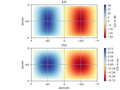
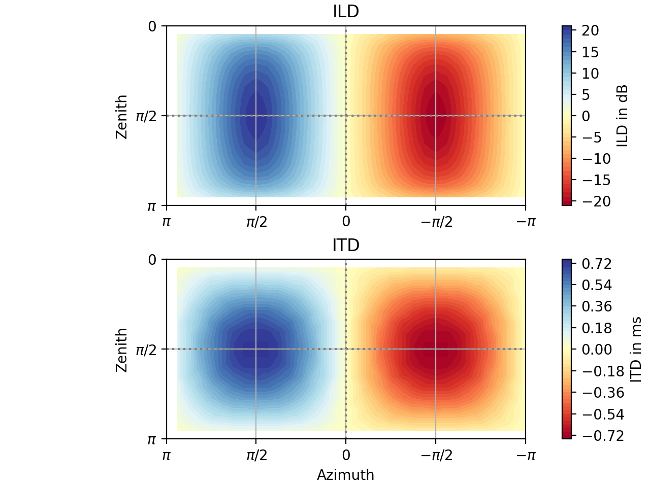
spaudiopy.plot.hrirs_ild_itd(hrirs, plevels=50, pclims=(None, None), title=None, fig=None)[source]

Plot ILDs and ITDs of HRIRs.

Parameters:

hrirs (sig.HRIRs)
plevels (int, optional) – Contour levels. The default is 50.
pclims ((2,), optional) – Set the plot color limits for ild and itd, e.g. (20, 0.75)
title (string, optional.)
fig (plt.figure, optional)

Returns:

None.